How to Use deMon2k
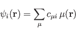
The deMon2k program implements DFT in the Kohn-Sham formulation. It uses the
linear combination of Gaussian type orbital (LCGTO) method. In this
framework, the Kohn-Sham orbitals
 are expanded in an
atomic
orbital basis:
are expanded in an
atomic
orbital basis:
 |
(1) |
Here
 denotes an atomic orbital (built from contracted
Gaussian basis functions) and
denotes an atomic orbital (built from contracted
Gaussian basis functions) and  the corresponding molecular orbital
coefficient. With this expansion, the electronic density is:
the corresponding molecular orbital
coefficient. With this expansion, the electronic density is:
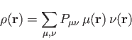 |
(2) |
 is an element of the (closed-shell, also called non-spin-polarized
in the DFT literature) density matrix defined as:
is an element of the (closed-shell, also called non-spin-polarized
in the DFT literature) density matrix defined as:
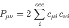 |
(3) |
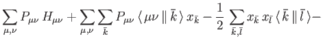
Using the LCGTO expansions for the Kohn-Sham orbitals (1.1) and
the electronic density (1.2), the Kohn-Sham self-consistent field
(SCF) energy expression [49] can be expressed as:
![\begin{displaymath}
E_{SCF} = \sum_{\mu , \nu} P_{\mu \nu} \, H_{\mu \nu} +
{1...
...\, \mu \nu \, \Vert \, \sigma \tau \, \rangle + E_{xc}[\rho]%
\end{displaymath}](ug-img15.png) |
(4) |
The total energy is the sum of  and the nuclear repulsion energy,
which can be calculated analytically. In (1.4),
and the nuclear repulsion energy,
which can be calculated analytically. In (1.4),  are elements of the core Hamiltonian matrix. They are built from the
kinetic and nuclear attraction energy operators of the electrons and describe
the distribution of an independent electron in the nuclear framework. The second
term in (1.4) is the Coulomb repulsion energy of the electrons. In
the short-hand notation for the four-center electron repulsion integrals
(ERIs) the symbol
are elements of the core Hamiltonian matrix. They are built from the
kinetic and nuclear attraction energy operators of the electrons and describe
the distribution of an independent electron in the nuclear framework. The second
term in (1.4) is the Coulomb repulsion energy of the electrons. In
the short-hand notation for the four-center electron repulsion integrals
(ERIs) the symbol  represents the two-electron Coulomb operator and
separates functions of electron 1 from those of electron 2.
In contrast to Hartree-Fock theory, the calculations of the Coulomb and
exchange energies are separate in Kohn-Sham DFT. Calculation of the
exchange-correlation energy
represents the two-electron Coulomb operator and
separates functions of electron 1 from those of electron 2.
In contrast to Hartree-Fock theory, the calculations of the Coulomb and
exchange energies are separate in Kohn-Sham DFT. Calculation of the
exchange-correlation energy ![$E_{xc}[\rho]$](ug-img19.png) requires numerical integration.
In deMon2k, the
requires numerical integration.
In deMon2k, the  scaling of straight-forward calculation of the Coulomb
repulsion energy is avoided by introducing an auxiliary function density
[50]. This approximated density
scaling of straight-forward calculation of the Coulomb
repulsion energy is avoided by introducing an auxiliary function density
[50]. This approximated density
 is expanded
in primitive Hermite Gaussians
is expanded
in primitive Hermite Gaussians
 which are centered on
the atoms [51,52]:
which are centered on
the atoms [51,52]:
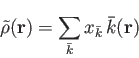 |
(5) |
The primitive Hermite Gaussian auxiliary functions are grouped in
auxiliary function sets that share the same exponent [53,54]. For
this reason, they usually are denoted as s, p, d etc. auxiliary
function sets. With the LCGTO expansion for
 and
and
 we obtain the following approximate SCF energy:
![\begin{displaymath}
E_{SCF} = \sum_{\mu , \nu} P_{\mu \nu} \, H_{\mu \nu} +
\s...
... \, {\bar k} \, \Vert \, {\bar l} \, \rangle} + E_{xc}[\rho]%
\end{displaymath}](ug-img26.png) |
(6) |
Therefore, only three-center electron repulsion integrals are necessary
for the SCF and energy calculation in deMon2k. This represents the density fitting
Kohn-Sham method available in deMon2k. It is activated by the keyword VXCTYPE
BASIS (see Section 4.2.1 for more details about the VXCTYPE keyword).
However, by default (VXCTYPE AUXIS), the approximated density is also used for
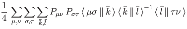
the calculation of the exchange-correlation energy:
![\begin{displaymath}
E_{SCF} = \sum_{\mu , \nu} P_{\mu \nu} \, H_{\mu \nu} +
\s...
...ar k} \, \Vert \, {\bar l} \, \rangle} + E_{xc}[\tilde \rho]%
\end{displaymath}](ug-img27.png) |
(7) |
This is the auxiliary density functional theory (ADFT) energy expression. For
more details on ADFT, see the reviews
[55,56,57,58,59]. Typically, the optimized ADFT
structure parameters are indistinguishable from their full DFT counterparts even
for weakly bound systems (here the use of the GEN-A2* auxiliary function set is
recommended; see Section 4.3.3 and Appendix A). For binding
energies, ADFT and Kohn-Sham results typically deviate by less than 1 kcal/mol
if GEN-A2* or larger auxiliary function sets are used. Thus, the differences
between ADFT and Kohn-Sham DFT geometries and bond energies are usually in the
range of the accuracy of the underlying approximate exchange-correlation
functional. Because of the considerable savings in computational time, we suggest
to use ADFT for all studies including frequency analysis and property calculations.
The VXCTYPE BASIS option Eq. (1.6) should be employed
only if direct comparison with four-center DFT calculations is required. It should
be noted that the default setting for the auxiliary functions is GEN-A2, independent
of which energy expression is used (see Section 4.3.3). For all theoretical
models available in deMon2k, VXCTYPE AUXIS results can be used as a restart guess
(GUESS RESTART; see Section 4.5.5) for VXCTYPE BASIS calculations.
The most frequently encountered problem in DFT calculations is the failure to
achieve SCF convergence. Usually this is caused by the small energy gap between the
highest occupied (HOMO) and lowest unoccupied (LUMO) molecular orbital. In
deMon2k, the DIIS procedure (Section 4.5.8) is activated by default. For a
small HOMO-LUMO gap, DIIS may be counterproductive and should be switched off.
There are several options available in deMon2k to achieve SCF convergence. Most
important are modifications of the choice of the starting GUESS (Section
4.5.5) and the MIXING (Section 4.5.6) of the old and new
(auxiliary) densities as well as enlargement of the HOMO-LUMO gap by the
level-SHIFT (Section 4.5.7) procedure. If a static level-shift is employed it
is advisable to check the orbital energies and occupations at the HOMO-LUMO
gap by use of the PRINT keyword (Section 4.12.2). Other relevant keywords to
alter or achieve SCF convergence are MOEXCHANGE (Section 4.4.3),
FIXMOS (Section 4.4.5) and SMEAR (Section 4.4.6). For atomic
calculations, the CONFIGURE keyword (Section 4.4.7) should be
used in order to ensure SCF convergence.
In deMon2k 5.0 the calculation of Hartree-Fock energies by the variational
fitting of the Coulomb and Fock potentials is also available. The corresponding
SCF energy has the form [43]:
Note that the same auxiliary function sets are used for the Coulomb and Fock
potential fitting. As a result, the approximated Hartree-Fock energy, Eq.
(1.8), is self-interaction free. To obtain a computationally
efficient methodology the Fock potential fitting is performed with localized molecular
orbitals [61]. This yields a computationally efficient and very accurate
approximate Hartree-Fock energy expression that only requires three-center ERIs.
Deviations with respect to four center ERIs total energies are below 1 kcal/mol
if GEN-A2* auxiliary function sets are used. With this development hybrid functionals
such as B3LYP [62,63], PBE0 [64,65] and M06-2X [66] are
now available in deMon2k [67].
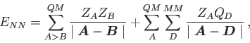
For QM/MM calculations in deMon2k 5.0 the following energy expression is used
[44]:
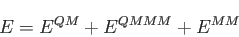 |
(9) |
The QM energy,  , can be calculated with any of the above discussed SCF energy
expressions given in Eqs. (1.6) to
(1.8) or corresponding hybrid functional expressions.
In all cases the core Hamiltonian matrix elements,
, can be calculated with any of the above discussed SCF energy
expressions given in Eqs. (1.6) to
(1.8) or corresponding hybrid functional expressions.
In all cases the core Hamiltonian matrix elements,  , are augmented in order
to take into account the electrostatic embedding of the QM system by the MM region:
, are augmented in order
to take into account the electrostatic embedding of the QM system by the MM region:
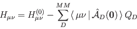 |
(10) |
In Eq. (1.10)
 denotes original core Hamilton matrix elements
of the QM system and
denotes original core Hamilton matrix elements
of the QM system and  denotes the atomic charges of the MM atoms
  . The general
form of the nuclear attraction type operator.
. The general
form of the nuclear attraction type operator.
 , is given by:
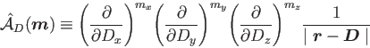 |
(11) |
This general definition permits immediately the inclusion of MM atoms with higher point
moments. Note that Eq. (1.10) is also used for pure electrostatic embedding
[68] with the EMBED keyword (see 4.2.6). In both cases asymptotic expansions
for the long-range nuclear attraction type integrals are implemented in order to improve
computational efficiency [69]. Another part of the QM energy in Eq.
(1.9) is the MM augmented nuclear repulsion energy,
which can be calculated analytically from the structure of the QM/MM system. Because the
so-defined QM energy contains all quantum mechanical terms plus the electrostatic
embedding from the MM region the Kohn-Sham or Hartree-Fock matrix elements can be
defined as partial derivatives of this energy with respect to density matrix elements.
The second term in Eq. (1.9) contains the mechanical interaction energy
between the QM and MM regions. It is expressed in the form of a Lennard-Jones potential:
![\begin{displaymath}
E^{QMMM} = \sum_A^{QM} \sum_D^{MM} \epsilon_{AD} \Biggl [
...
...math$A$} - \mbox{\boldmath$D$} \mid}} \right )}^{6} \Biggr ]%
\end{displaymath}](ug-img42.png) |
(12) |
The  are combinations of the van der Waals radii of QM atom
  and MM atom
  .
By default these radii are taken from the MM force field. The parameter
.
By default these radii are taken from the MM force field. The parameter  defines the depth of the Lennard-Jones potential. As for the van der Waals radii it is
also taken from the MM force field. Therefore, an MM atom type has to be assigned to
each QM atom in the input. This is done with the QM/MM keyword (Section 4.2.4).
defines the depth of the Lennard-Jones potential. As for the van der Waals radii it is
also taken from the MM force field. Therefore, an MM atom type has to be assigned to
each QM atom in the input. This is done with the QM/MM keyword (Section 4.2.4).
The last term in Eq. (1.9) is the MM energy. In deMon2k 5.0 it can contain
the following terms:
 |
(13) |
The first four terms in Eq. (1.14) denote bond stretching, angle bending,
dihedral torsion and Urey-Bradley energy terms. Their calculation requires molecular
connectivity information that is usually given in the input along with the geometrical
definition of the MM atoms under the GEOMETRY keyword (see 4.1.1). As an
alternative, the automatic generation of molecular connectivity information on the
basis of the distances between MM atoms is also available. The last two terms in
Eq. (1.14) represent van der Waals and point-charge interaction energies
between the MM atoms. The force fields for MM and QM/MM calculations available in
deMon2k are OPLS-AA [45] and AMBER [70]. They are selected by the
FORCEFIELD keyword (see 4.2.3) and read from the FFDS (force field dataset)
file. For these MM and QM/MM calculations all deMon2k functionalities, such as
geometry optimization, transition state finding, molecular dynamics, frequency
analysis etc., are available. Also property calculations for the QM system in
QM/MM calculations are possible [71].
Besides the internal MM capability, deMon2k can also be externally interfaced with
force fields. To this end a standard interface output for CHARMM [72] can
be activated with the QM/MM keyword [44,46,73].
By default, the ERIs are calculated in each SCF cycle (direct SCF) using recurrence
relations for near-field ERIs [20,51] and double asymptotic expansions [74]
for far-field ERIs. This approach minimizes the random access memory (RAM) demand of
deMon2k. If sufficient RAM is available the code performance can be improved by the
MIXED option of the ERIS keyword (see 4.5.4). The RAM usage of deMon2k can be
monitored by PRINT RAM (see Section 4.12.2 for more details). It also should
be noted that, for larger systems, the linear algebra steps in deMon2k may become
a bottleneck. With the keywords MATDIA and MATINV (see 4.11.2 and 4.11.3)
alternative diagonalizers and matrix inversion techniques can be selected.
Several optimization and transition state search algorithms are
implemented in deMon2k. For structure optimization, the default setting is
the Levenberg-Marquardt restricted step method in delocalized internal
redundant coordinates. This method has excellent convergence
behavior and is very robust. However, it requires an iterative back
transformation of the coordinates. Thus, to reach tight structure convergence,
it may be necessary to switch to Cartesian coordinates at the end of the
optimization (see 4.6.1). For ultimate accuracy, this
might be combined with a Hessian calculation in each optimization step
(UPDATE EXACT; Section 4.6.5). If effective core potentials (ECPs),
Section 4.3.4, or model core potentials (MCPs), Section 4.3.5, are used,
care must be taken regarding the accuracy of the gradients. Here it may be necessary
to tighten the numerical integration threshold with the GRID keyword
(see 4.3.6). Usually a FINE grid will be sufficient. The same holds
for weak and nonbonded interactions. For the local transition state search,
we recommend starting the optimization from a calculated Hessian
(see 4.6.5) or restarting it from a frequency analysis (the Hessian
from the frequency analysis is then used in the first optimization step).
If a SADDLE point interpolation (Section 4.6.2) is to be performed,
the starting points must be local minima, i.e. reactants and products.
All optimizations
and interpolations can be restarted with the deMon.new and
deMon.mem files. These must be copied into the new input file
deMon.inp and the corresponding restart file deMon.rst. The
new input file may be modified and extended but the molecular geometry
definitions must be left untouched in order to guarantee a successful
restart run.
Born-Oppenheimer molecular dynamics (BOMD) simulations are initialized by the
DYNAMICS keyword (see 4.7.1). In these calculations a trajectory
file deMon.trj is created which can be large! For compatibility
reasons, the trajectory file is written in ASCII
(Note that *********************** are used as separations in this file).
It should not be modified.
The data from the trajectory file can be used to restart BOMD runs or to
analyze them (Sections 4.7.2 and 4.7.3). Because BOMD
runs may take weeks, we recommend that regular snapshots of the deMon working
directory be produced from which restarts are possible. During such a copy the
trajectory, deMon.trj, and new input file, deMon.new, must
be unchanged. With these files, a restart run is possible just as in the case of
structure optimizations, i.e. the deMon.new must be copied into
the new input file deMon.inp. If requested, the restart file can also
be used, e.g. for a restart density (GUESS RESTART; see 4.5.5).
However, this is not mandatory.
Usually the default settings of deMon2k are sufficient for standard calculations.
However, if extended basis sets are used or higher accuracy is required, it may be
necessary to adjust the accuracy and performance settings of the code. This is
achieved by the keywords GRID, SCFTYPE and ERIS (see 4.3.6, 4.5.1
and 4.5.4) for the electronic structure calculation, the keyword OPTIMIZATION
(see 4.6.1) for the structure optimization and the keywords MATDIA
and MATINV (see 4.11.2 and 4.11.3) for the linear algebra parts of the
code. The keywords WEIGHTING, QUADRATURE and CFPINTEGRATION control the
accuracy settings for the numerical integration (see 4.11.5,
4.11.6 and 4.11.7). The keyword DAVIDSON
(4.11.4) controls the iterative diagonalization in time-dependent
DFT calculations. In general, modification of the standard settings may
alter the performance and accuracy of the code quite substantially.
Therefore, such modifications should be tested carefully before being
used for production runs.