Keyword SCFTYPE

With this keyword the SCF method is selected and SCF convergence control is specified.
Options:
RKS / UKS / ROKS / CUKS

	RKS		The restricted Kohn-Sham method will be used. This is the default for closed-shell systems.
	UKS		The unrestricted Kohn-Sham method will be used. This is the default for open-shell systems.
	ROKS		The spin-restricted open-shell Kohn-Sham method will be used.
	$<$ROKS option$>$		The ROKS option string defines the ROKS parametrization according to Table 8. By default the Guest & Saunders parametrization [174] is used.
	CUKS		The constrained unrestricted Kohn-Sham method will be used.
	MAX=$<$Integer$>$		Maximum number of SCF iterations. Default is 100.
	TOL=$<$Real$>$		MinMax SCF energy convergence criterion. Default is $10^{-5}$ a.u.
	CDF=$<$Real$>$		Auxiliary density convergence criterion. Default is $5 \cdot 10^{-4}$ a.u.
	NOTIGHTEN		The SCF convergence criteria will not be adjusted during an optimization, frequency analysis or property calculation.

Description:
The implementations of the Kohn-Sham SCF methods are similar to the corresponding Hartree-Fock methods [166,167,168,169,170] and have similar advantages and disadvantages. For historical reasons the three-center ERI Hartree-Fock methods are also selected by the RKS, UKS, ROKS and CUKS options of the SCFTYPE keyword. In the case of UKS calculations, spin-contamination may appear. In deMon2k, the approximate spin contamination [171,172] is calculated and printed just before the converged UKS SCF energy. This printed value has proven to be a good guide for evaluation of spin-contamination in UKS calculations. The ROKS implementation [173] in deMon2k follows the original Roothaan work for Hartree-Fock [169]. Six different parametrizations for the mixing factors of the diagonal blocks of the ROKS Kohn-Sham matrix,

$$\pmatrix{ {\mbox{\boldmath$K$}}^2 & {\mbox{\boldmath$K$}}^... ...boldmath$K$}}^{\alpha} & {\mbox{\boldmath$K$}}^0 \cr } \> ,%$$ (12)

where ${\mbox{\boldmath$K$}}^{\alpha}$ and ${\mbox{\boldmath$K$}}^{\beta}$ are the usual $\alpha$ and $\beta$ Kohn-Sham matrices in MO representation and ${\mbox{\boldmath$K$}}^2$, ${\mbox{\boldmath$K$}}^1$ and ${\mbox{\boldmath$K$}}^0$ are the diagonal blocks for double, single and unoccupied MOs, are implemented in deMon2k. The corresponding mixing equations are given by: @fnswfnvalfnswfalse ##1fnval##1fnswtrue

$${\mbox{\boldmath$K$}}^2 = A_2 {\mbox{\boldmath$K$}}^{\alpha} + B_2 {\mbox{\boldmath$K$}}^{\beta}$$ (13)

$${\mbox{\boldmath$K$}}^1 = A_1 {\mbox{\boldmath$K$}}^{\alpha} + B_1 {\mbox{\boldmath$K$}}^{\beta}$$ (14)

$${\mbox{\boldmath$K$}}^0 = A_0 {\mbox{\boldmath$K$}}^{\alpha} + B_0 {\mbox{\boldmath$K$}}^{\beta}$$ (15)

The mixing factors of the different parametrizations [175] along with their SCFTYPE keyword options are given in Table 8.

Table 8: Mixing factors and SCFTYPE options of the ROKS parametrizations available in deMon2k.

$$A_0 B_0 A_1 B_1 A_2 B_2$$ Parametrization SCFTYPE option

$$1/2 1/2 1/2 1/2 1/2 1/2$$ Guest & Saunders [174] GUEST (default)

$$3/2 1/2 1/2 1/2 1/2 3/2$$ Roothaan [169] ROOTHAAN

$$1 0 1 0 1/2 1/2$$ Davidson [176] DAVIDSON

$$0 1 1 0 1/2 1/2$$ Binkley et al. [170] BINKLEY

$$2/3 1/3 1/3 1/3 1/3 2/3$$ McWeeny & Diercksen [177] MCWEENY

$$1/2 1/2 1 0 1/2 1/2$$ Faegri & Manne [178] FAEGRI

$$1 0 1 0 0 1$$ Plakhutin et al. [175] PLAKHUTIN

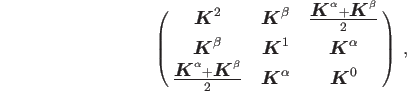
Note that the ROKS orbital energies vary with respect to these parametrizations and, therefore, are not uniquely defined. In particular, the Aufbau principle for the doubly and singly occupied molecular orbital energy manifolds can be violated [179,180]. Moreover, ROKS orbital energies include additional constraints and cannot be compared with RKS or UKS orbital energies. Specifically, the Slater-Janak theorem [181,182] does not hold for ROKS calculations. For this reason the block-diagonalized ROKS $\alpha$ and $\beta$ MO energies and coefficients [183], also named semi-canonical spin orbitals, are printed after the ROKS energy as shown in the following example output for a B3LYP/STO-3G/GEN-A2* calculation of the triplet O$_2$ ground state.

 *** SCF CONVERGED ***


 MO COEFFICIENTS OF CYCLE 7


                                7          8          9         10
                            -0.3794    -0.0601    -0.0601     0.4267
 
                             2.0000     1.0000     1.0000     0.0000
 
     1    1   O    1s        0.0000     0.0000     0.0000    -0.0917
     2    1   O    2s        0.0000     0.0000     0.0000     0.5671
     3    1   O    2py       0.6576     0.0822     0.7637     0.0000
     4    1   O    2pz       0.0000     0.0000     0.0000     0.9484
     5    1   O    2px       0.0374     0.7637    -0.0822     0.0000
 
     6    2   O    1s        0.0000     0.0000     0.0000     0.0917
     7    2   O    2s        0.0000     0.0000     0.0000    -0.5671
     8    2   O    2py       0.6576    -0.0822    -0.7637     0.0000
     9    2   O    2pz       0.0000     0.0000     0.0000     0.9484
    10    2   O    2px       0.0374    -0.7637     0.0822     0.0000


 
 RANDOMIZED SCF GRID GENERATED IN 3 CYCLES
 

 REFERENCE VALUE OF S**2 FOR PURE SPIN STATE S(S+1):    2.0000

 S**2 BEFORE SPIN PROJECTION:    2.0000
 S**2 AFTER SPIN PROJECTION:     2.0000


 ELECTRONIC CORE ENERGY      =       -260.328412563
 ELECTRONIC COULOMB ENERGY   =        101.099784250
 ELECTRONIC HARTREE ENERGY   =       -159.228628313

 EXCHANGE ENERGY             =        -16.350046036
 CORRELATION ENERGY          =         -0.733801619
 EXCHANGE-CORRELATION ENERGY =        -17.083847655

 ELECTRONIC SCF ENERGY       =       -176.312475968
 NUCLEAR-REPULSION ENERGY    =         28.059106307
 TOTAL ENERGY                =       -148.253369660



 BLOCK DIAGONAL ALPHA MO COEFFICIENTS


                                7          8          9         10
                            -0.4028    -0.1618    -0.1618     0.4020
 
                             1.0000     1.0000     1.0000     0.0000
 
     1    1   O    1s        0.0729     0.0000     0.0000    -0.0917
     2    1   O    2s       -0.3516     0.0000     0.0000     0.5671
     3    1   O    2py       0.0000    -0.7148    -0.2813     0.0000
     4    1   O    2pz       0.6083     0.0000     0.0000     0.9484
     5    1   O    2px       0.0000     0.2813    -0.7148     0.0000
 
     6    2   O    1s        0.0729     0.0000     0.0000     0.0917
     7    2   O    2s       -0.3516     0.0000     0.0000    -0.5671
     8    2   O    2py       0.0000     0.7148     0.2813     0.0000
     9    2   O    2pz      -0.6083     0.0000     0.0000     0.9484
    10    2   O    2px       0.0000    -0.2813     0.7148     0.0000




 BLOCK DIAGONAL BETA MO COEFFICIENTS


                                7          8          9         10
                            -0.3239     0.0415     0.0415     0.4515
 
                             1.0000     0.0000     0.0000     0.0000
 
     1    1   O    1s        0.0000     0.0000     0.0000    -0.0917
     2    1   O    2s        0.0000     0.0000     0.0000     0.5671
     3    1   O    2py      -0.3948    -0.7637    -0.0825     0.0000
     4    1   O    2pz       0.0000     0.0000     0.0000     0.9484
     5    1   O    2px       0.5272     0.0825    -0.7637     0.0000
 
     6    2   O    1s        0.0000     0.0000     0.0000     0.0917
     7    2   O    2s        0.0000     0.0000     0.0000    -0.5671
     8    2   O    2py      -0.3948     0.7637     0.0825     0.0000
     9    2   O    2pz       0.0000     0.0000     0.0000     0.9484
    10    2   O    2px       0.5272    -0.0825     0.7637     0.0000

The printing of the MO energies and coefficients is activated with PRINT MOS=7-10 (see Section 4.12.2). The block diagonal $\alpha$ and $\beta$ MO energies and coefficients can be directly compared with their UKS counterparts. In deMon2k they are also used for ROKS perturbation theory calculations. As an alternative to ROKS the constrained unrestricted Kohn-Sham (CUKS) method can be used for spin-projection [184] where the semi-canonical orbitals are obtained directly. The convergence behavior of ROKS and CUKS calculations is generally different and it is advisable to switch among them to test convergence in problematic cases.

As a consequence of the variational fitting of the density [5,6], deMon2k can exploit a MinMax SCF procedure [185]. In a variational MinMax procedure, there is no strict convergence from above. Therefore, it is possible to obtain energies below the converged energy during the SCF iterations in deMon2k. Note that the printed SCF ERROR for an SCF cycle is the difference between upper and lower MinMax energy bounds and, thus, a direct measurement of how far the current SCF step is away from the convergence point.

The maximum number of SCF iterations is specified with the MAX option. With MAX=0 an "energy only" calculation with the molecular orbital coefficients from the restart file can be performed. No SCF iteration is done! The MAX=0 option automatically triggers GUESS RESTART (see 4.5.5) and, therefore, fails if no adequate restart file deMon.rst exists. The ordering and, thus, the occupation of the molecular orbitals in the restart file can be altered with the MOEXCHANGE keyword (see Section 4.4.3).

The SCF energy convergence criterion can be defined by the user with the TOL option. Such a user-defined SCF convergence criterion is valid for the first single-point SCF calculation. During a geometry optimization, however, the convergence criterion is automatically tightened according to the residual forces (see Table 9). However, if the user-defined convergence criterion is smaller than the automatic-tightening value, the user-defined value is used instead. If self-consistent perturbation calculations are performed, the automatically requested SCF energy convergence criterion is $10^{-6}$ Hartree. It too may be overridden by a smaller value with the TOL option.

Table 9: Tightening of the SCF convergence criteria during structure optimization.

RMS Gradient [a.u] TOL[a.u.] CDF

$$\leq 0.02 1.0 \cdot 10^{-5\phantom{0}} 1.0 \cdot 10^{-3}$$

$$\leq 0.01 5.0 \cdot 10^{-6\phantom{0}} 5.0 \cdot 10^{-4}$$

$$\leq 0.005 1.0 \cdot 10^{-7\phantom{0}} 1.0 \cdot 10^{-4}$$

$$\leq 0.001 7.5 \cdot 10^{-8\phantom{0}} 7.5 \cdot 10^{-5}$$

$$\leq 7.5 \cdot 10^{-4} 5.0 \cdot 10^{-8\phantom{0}} 5.0 \cdot 10^{-5}$$

$$\leq 5.0 \cdot 10^{-4} 2.5 \cdot 10^{-8\phantom{0}} 2.5 \cdot 10^{-5}$$

$$\leq 1.0 \cdot 10^{-4} 1.0 \cdot 10^{-8\phantom{0}} 1.0 \cdot 10^{-5}$$

$$\leq 7.5 \cdot 10^{-5} 7.5 \cdot 10^{-9\phantom{0}} 7.5 \cdot 10^{-6}$$

$$\leq 5.0 \cdot 10^{-5} 5.0 \cdot 10^{-9\phantom{0}} 5.0 \cdot 10^{-6}$$

$$\leq 2.5 \cdot 10^{-5} 2.5 \cdot 10^{-9\phantom{0}} 2.5 \cdot 10^{-6}$$

$$\leq 1.0 \cdot 10^{-5} 1.0 \cdot 10^{-9\phantom{0}} 1.0 \cdot 10^{-6}$$

$$\leq 7.5 \cdot 10^{-6} 7.5 \cdot 10^{-10} 7.5 \cdot 10^{-7}$$

$$\leq 5.0 \cdot 10^{-6} 5.0 \cdot 10^{-10} 5.0 \cdot 10^{-7}$$

$$\leq 2.5 \cdot 10^{-6} 2.5 \cdot 10^{-10} 2.5 \cdot 10^{-7}$$

$$\leq 1.0 \cdot 10^{-6} 1.0 \cdot 10^{-10} 1.0 \cdot 10^{-7}$$

$$\leq 7.5 \cdot 10^{-7} 1.0 \cdot 10^{-10} 7.5 \cdot 10^{-8}$$

$$\leq 5.0 \cdot 10^{-7} 1.0 \cdot 10^{-10} 5.0 \cdot 10^{-8}$$

$$\leq 2.5 \cdot 10^{-7} 1.0 \cdot 10^{-10} 2.5 \cdot 10^{-8}$$

The auxiliary density convergence criterion can be defined by the user with the CDF option. As with the user-defined energy convergence criterion, the user-defined auxiliary density convergence criterion holds for the first single-point SCF calculation and overrides the automatically determined CDF values (see Table 9) during the optimization if the user-defined value is smaller. If self-consistent perturbation calculations are performed, the default auxiliary density convergence criterion is tightened to $5 \cdot 10^{-5}$. Again, this value can be overridden by a smaller user-defined value with the CDF option. At SCF convergence both energy and auxiliary density convergence criteria are satisfied.

The option NOTIGHTEN disables the automatic tightening of the SCF convergence criteria according to the root mean square (RMS) gradient (as shown in Table 9). Thus, the SCF convergence tolerance is relaxed during geometry optimization and, therefore, SCF convergence failures are less likely. However, accuracy of the gradients is compromised and the structural optimization may not converge. Good practice, therefore, is to use NOTIGHTEN only at the beginning of the optimization or in combination with carefully tested user-defined TOL and CDF values. The NOTIGHTEN option also disables tightening of SCF convergence for perturbation calculations.